Performance of Modern Java on Data-Heavy Workloads: Real-Time Streaming

This post is a part of a series:

• Part 1 (you are here)
• Part 2 (batch workload benchmark)
• Part 3 (low-latency benchmark)
• Part 4 (concurrent GC with green threads)
• Part 5 (billion events per second)

The Java runtime has been evolving more rapidly in recent years and, after 15 years, we finally got a new default garbage collector: the G1. Two more GCs are on their way to production and are available as experimental features: Oracle's ZGC and OpenJDK's Shenandoah.

We at Hazelcast thought it was time to put all these new options to the test and find which choices work well with workloads typical for our distributed stream processing engine, Hazelcast Jet.

Jet is being used for a broad spectrum of use cases, with different latency and throughput requirements. Here are three important categories:

1. Low-latency unbounded stream processing, with moderate state. Example: detecting trends in 100 Hz sensor data from 10,000 devices and sending corrective feedback within 10-20 milliseconds.
2. High-throughput, large-state unbounded stream processing. Example: tracking GPS locations of millions of users, inferring their velocity vectors.
3. Old-school batch processing of big data volumes. The relevant measure is time to complete, which implies a high throughput demand. Example: analyzing a day's worth of stock trading data to update the risk exposure of a given portfolio.

At the outset, we can observe the following:

• in scenario 1 the latency requirements enter the danger zone of GC pauses: 100 milliseconds, something traditionally considered an excellent result for a worst-case GC pause, may be a showstopper for many use cases
• scenarios 2 and 3 are similar in terms of demands on the garbage collector. Less strict latency, but large pressure on the tenured generation
• scenario 2 is tougher because latency, even if less so than in scenario 1, is still relevant

We tried the following combinations:

1. JDK 8 with the default Parallel collector and the optional ConcurrentMarkSweep and G1
2. JDK 11 with the default G1 collector and the optional Parallel
3. JDK 14 with the default G1 as well as the experimental ZGC and Shenandoah

And here are our overall conclusions:

1. On modern JDK versions, the G1 is one monster of a collector. It handles heaps of dozens of GB with ease (we tried 60 GB), keeping maximum GC pauses within 200 ms. Under extreme pressure it doesn't show brittleness with catastrophic failure modes. Instead the Full GC pauses rise into the low seconds range. Its Achilles' heel is the upper bound on the GC pause in favorable low-pressure conditions, which we couldn't push lower than 20-25 ms.
2. JDK 8 is an antiquated runtime. The default Parallel collector enters huge Full GC pauses and the G1, although having less frequent Full GCs, is stuck in an old version that uses just one thread to perform it, resulting in even longer pauses. Even on a moderate heap of 12 GB, the pauses were exceeding 20 seconds for Parallel and a full minute for G1. The ConcurrentMarkSweep collector is strictly worse than G1 in all scenarios, and its failure mode are multi-minute Full GC pauses.
3. The ZGC, while allowing substantially less throughput than G1, was very good in that one weak area of G1, occasionally increasing our latency by up to 10 ms under light load.
4. Shenandoah was a disappointment with occasional, but nevertheless regular, latency spikes up to 220 ms in the low-pressure regime.
5. Neither ZGC nor Shenandoah showed as smooth failure modes as G1. They exhibited brittleness, with the low-latency regime suddenly giving way to very long pauses and even OOMEs.

This post is Part 1 of a two-part series and presents our findings for the two streaming scenarios. In Part 2, we'll present the results for batch processing.

Streaming Pipeline Benchmark

For the streaming benchmarks, we used the code available here, with some minor variations between the tests. Here is the main part, the Jet pipeline:

StreamStage<Long> source = p.readFrom(longSource(ITEMS_PER_SECOND))
                            .withNativeTimestamps(0)
                            .rebalance(); // Introduced in Jet 4.2
source.groupingKey(n -> n % NUM_KEYS)
      .window(sliding(SECONDS.toMillis(WIN_SIZE_SECONDS), SLIDING_STEP_MILLIS))
      .aggregate(counting())
      .filter(kwr -> kwr.getKey() % DIAGNOSTIC_KEYSET_DOWNSAMPLING_FACTOR == 0)
      .window(tumbling(SLIDING_STEP_MILLIS))
      .aggregate(counting())
      .writeTo(Sinks.logger(wr -> String.format("time %,d: latency %,d ms, cca. %,d keys",
              simpleTime(wr.end()),
              NANOSECONDS.toMillis(System.nanoTime()) - wr.end(),
              wr.result() * DIAGNOSTIC_KEYSET_DOWNSAMPLING_FACTOR)));

This pipeline represents use cases with an unbounded event stream where the engine is asked to perform sliding window aggregation. You need this kind of aggregation, for example, to obtain the time derivative of a changing quantity, remove high-frequency noise from the data (smoothing) or measure the intensity of the occurrence of some event (events per second). The engine can first split the stream by some category (for example, each distinct IoT device or smartphone) into substreams and then independently track the aggregated value in each of them. In Hazelcast Jet the sliding window moves in fixed-size steps that you configure. For example, with a sliding step of 1 second you get a complete set of results every second, and if the window size is 1 minute, the results reflect the events that occurred within the last minute.

Some notes:

• The code is entirely self-contained with no outside data sources or sinks. We use a mock data source that simulates an event stream with exactly the chosen number of events per second. Consecutive event timestamps are an equal amount of time apart. The source never emits an event whose timestamp is still in the future, but otherwise emits them as fast as possible.
• If the pipeline falls behind, events will be "buffered" but without any storage. After falling behind, the pipeline must catch up by ingesting data as fast as it can. Since our source is non-parallel, the limit on its throughput was about 2.2 million events per second. We used 1 million simulated events per second, leaving a catching-up headroom of 1.2 million per second.
• The pipeline measures its own latency by comparing the timestamp of an emitted sliding window result with the actual wall-clock time. In more detail, there are two aggregation stages with filtering between them. A single sliding window result consists of many items, each for one substream, and we're interested in the latency of the last-emitted item. For this reason we first filter out most of the output, keeping every 10,000th entry, and then direct the thinned-out stream to the second, non-keyed tumbling window stage that notes the result size and measures the latency. Non-keyed aggregation is not parallelized, so we get a single point of measurement. The filtering stage is parallel and data-local so the impact of the additional aggregation step is very small (well below 1 ms).
• We used a trivial aggregate function: counting, in effect obtaining the events/second metric of the stream. It has minimal state (a single
  long number) and produces no garbage. For any given heap usage in gigabytes, such a small state per key implies the worst case for the garbage collector: a very large number of objects. GC overheads scale much more with object count than heap size. We also tested a variant that computes the same aggregate function, but with a different implementation that produces garbage.
• We performed most of the streaming benchmarks on a single node since our focus was the effect of memory management on pipeline performance and network latency just adds noise into the picture. We repeated some key tests on a three-node Amazon EC2 cluster to validate our prediction that cluster performance won't affect our conclusions. You can find a more detailed justification for this towards the end of Part 2.
• We excluded the Parallel collector from the results for streaming workloads because the latency spikes it introduces would be unacceptable in pretty much any real-life scenario.

Scenario 1: Low Latency, Moderate State

For the first scenario we used these parameters:

• OpenJDK 14
• JVM heap size 4 gigabytes
• for G1, -XX:MaxGCPauseMillis=5
• 1 million events per second
• 50,000 distinct keys
• 30-second window sliding by 0.1 second

In this scenario there's less than 1 GB heap usage. The collector is not under high pressure, it has enough time to perform concurrent GC in the background. These are the maximum pipeline latencies we observed with the three garbage collectors we tested:

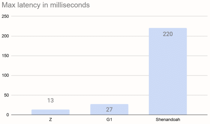
Note that these numbers include a fixed time of about 3 milliseconds to emit the window results. The chart is pretty self-explanatory: the default collector, G1, is pretty good on its own, but if you need even better latency, you can use the experimental ZGC collector. We couldn't reduce the latency spikes below 10 milliseconds, however we did note that, in the case of ZGC and Shenandoah, they weren't due to outright GC pauses but rather short periods of increased background GC work. Shenandoah's overheads occasionally raised latency above 200 ms.

Scenario 2: Large State, Less Strict Latency

In scenario 2 we assume that, for various reasons outside our control, (e.g., mobile network), the latency can grow into low seconds, which relaxes the requirements we must impose on our stream processing pipeline. On the other hand, we may be dealing with much larger data volumes, on the order of millions or dozens of millions of keys.

In this scenario we can provision our hardware so it's heavily utilized, relying on the GC to manage a large heap instead of spreading out the data over many cluster nodes.

We performed many tests with different combinations to find out how the interplay between various factors causes the runtime to either keep up or fall behind. In the end we found two parameters that determine this:

1. number of entries stored in the aggregation state
2. demand on the catching-up throughput

The first one corresponds to the number of objects in the tenured generation. Sliding window aggregation retains objects for a significant time (the length of the window) and then releases them. This goes directly against the Generational Garbage Hypothesis, which states that objects will either die young or live forever. This regime puts the strongest pressure on the GC, and since the GC effort scales with the number of live objects, performance is highly sensitive to this parameter.

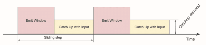
The second parameter relates to how much GC overhead the application can tolerate. To explain it better, let's use some diagrams. A pipeline performing windowed aggregation goes through three distinct steps:

1. processing events in real time, as they arrive
2. emitting the sliding window results
3. catching up with the events received while in step 2

The three phases can be visualized as follows:

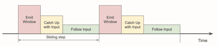
If emitting the window result takes longer, we get a situation like this:

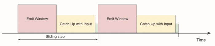
Now the headroom has shrunk to almost nothing, the pipeline is barely keeping up, and any temporary hiccups like an occasional GC pause will cause latency to grow and recover at a very slow pace.

If we change this picture and present just the average event ingestion rate after window emission, we get this:

We call the height of the yellow rectangle "catchup demand": it is the demand on the throughput of the source. If it exceeds the actual maximum throughput, the pipeline fails.

This is how it would look if window emission took way too long:

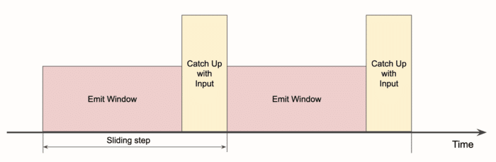
The area of the red and the yellow rectangles is fixed, it corresponds to the amount of data that must flow through the pipeline. Basically, the red rectangle "squeezes out" the yellow one. But the yellow rectangle's height is actually limited, in our case to 2.2 million events per second. So whenever it would be taller than the limit, we'd have a failing pipeline whose latency grows without bounds.

We worked out the formulas that predict the sizes of the rectangles for a given combination of event rate, window size, sliding step and keyset size, so that we could determine the catchup demand for each case.

Now that we have two more-or-less independent parameters derived from many more parameters describing each individual setup, we can create a 2D-chart where each benchmark run has a point on it. We assigned a color to each point, telling us whether the given combination worked or failed. For example, for JDK 14 with G1 on a developer's laptop, we got this picture:

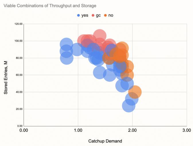
We made the distinction between "yes", "no" and "gc", meaning the pipeline keeps up, doesn't keep up due to lack of throughput, or doesn't keep up due to frequent long GC pauses. Note that the lack of throughput can also be caused by concurrent GC activity and frequent short GC pauses. In the end, the distinction doesn't matter a lot.

You can make out a contour that separates the lower-left area where things work out from the rest of the space, where they fail. We made the same kind of chart for other combinations of JDK and GC, extracted the contours, and came up with this summary chart:

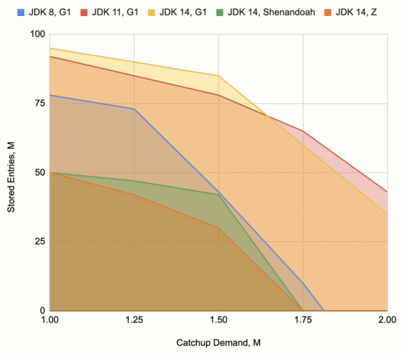
For reference, the hardware we used is a MacBook Pro 2018 with a 6-core Intel Core i7 and 16 GB DDR4 RAM, configuring -Xmx10g for the JVM. However, we do expect the overall relationship among the combinations to remain the same on a broad range of hardware parameters. The chart visualizes the superiority of the G1 over others, the weakness of the G1 on JDK 8, and the weakness of the experimental low-latency collectors for this kind of workload.

The base latency, the time it takes to emit the window results, was in the ballpark of 500 milliseconds, but latency would often take hikes due to occasional Major GC's (which are not unreasonably long with the G1), up to 10 seconds in the borderline cases (where the pipeline barely keeps up), and still recover back to a second or two. We also noticed the effects of JIT compilation in the borderline cases: the pipeline would start out with a constantly increasing latency, but then after around two minutes, its performance would improve and the latency would make a full recovery.

Go to Part 2: the Batch Pipeline Benchmarks.

If you enjoyed reading this post, check out Jet at GitHub and give us a star!