Aggregation Optimization in MongoDB: A Case Study From the Field (Part 1)

And why MongoDB might be a better relational database than you ever realized.

This article was written by Graeme Robinson. Find him on LinkedIn.

Design reviews are one-on-one meetings where MongoDB experts deliver advice on data modeling best practices and application design challenges. In this series, we are going to explore common real-life scenarios where design reviews helped developers achieve meaningful success with MongoDB.

---

MongoDB is often described as a non-relational database, but whenever we store data in a database, there are relationships within that data. Depending on the type of database we use, though, how we model those relationships may change. As my colleague Rick Houlihan has often pointed out, there really is no such thing as non-relational data.

MongoDB, by virtue of its use of the document data model rather than the rows and columns of tabular RDBMSs, provides ways of modeling relationships that can offer significant performance benefits when querying that data. However, to realize those benefits, data must be modeled in  MongoDB using schema design patterns that are optimized for the document data model, and frequently, those are not the same as would be appropriate in a RDBMS.

During a recent design review, I came across exactly that problem—a team relatively new to MongoDB had modeled their data in a very "RDBMS-like" manner and were struggling with poor query performance. However, with a relatively small set of changes to their data model and corresponding query design, we were able to transform their query, making it over 800 times faster than their initial design.

In this series of articles, we'll present a fictional scenario using a data model and aggregation pipeline query design based on that which was encountered during the review. We’ll then walk through each of the steps taken to improve the query performance, using the sample data set to show the impact of each step as we go.

If you wish to repeat the testing described in this series, the source code used to build the test data set and then measure the performance of each modification is available on GitHub.

The video streaming service use case: profiles, devices, and device types

For our example scenario, we created a database for a fictional video streaming service. The part of the system we were focused on dealt with user profiles and devices and contained three collections:

User “profiles” represented individual users accessing the streaming service. Each profile document contained a profile ID, the user’s name, date of birth and SSN, a contact address and telephone number, and the account number to which the profile belonged. (Each account could have multiple profiles. For example, a family might have one account with a separate profile for each family member.)

“Devices” were the devices used by profiles to access the streaming service. Each device document contained a serial number uniquely identifying the device, a device model name—for example, “iPhone 12” or “Amazon Fire Tablet”—the IP address from which the device last connected, and a date after which the device’s authorization to connect to the service would need to be renewed. 

A many-to-many relationship existed between devices and profiles — some devices, like smart TVs, tended to be used by all profiles associated with an account, while others, like smartphones, tended to be used by a single profile. Typically, each profile would access the service through more than one device. 

To map profiles to devices, an intermediate (or “associative”) "mappings" collection was used. Documents in this collection contained the profile ID of a profile at one side of the relationship and the device serial number of a device at the other side of the relationship, effectively turning the many-to-many relationship between profiles and devices into a one-to-many relationship between profiles and mappings, and a many-to-one relationship between mappings and devices.

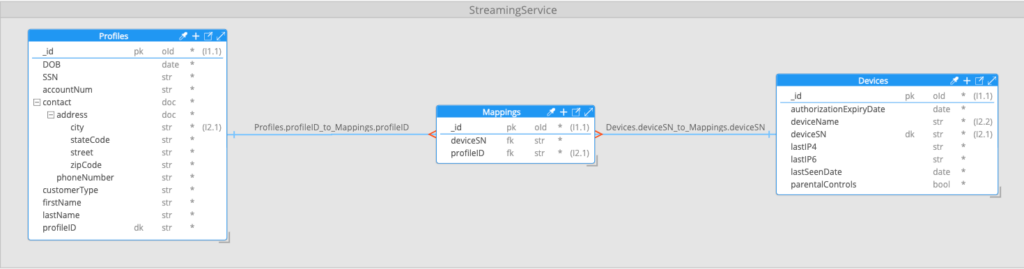
This approach to modeling many-to-many relationships is common when working with relational databases and works around the limitation that, with a tabular data model, there is no great way to store an arbitrary number of reference field values—in this case, profile IDs within devices, or device IDs within profiles.

Using this data model, the query that we were trying to perform was designed to provide a list of all profiles with an address in a given city, and that had used a specific device type to access the service—for example, all profiles with an address in Austin that had used an iPhone 12 to access the service. The output from the query was required to embed details of each device of the specified type used by a matching profile. Profiles were to be returned ordered by profile ID and in pages of 10 documents. An example output document would look like this:

{
  "SSN": "438-40-3508",
  "contact": {
    "address": {
      "city": "Austin",
      "stateCode": "TX",
      "street": "9590 Reagan Expressway",
      "zipCode": "84880"
    },
    "phoneNumber": "(834) 392-0946"
  },
  "firstName": "Sean",
  "lastName": "Henderson",
  "profileID": "R3G6RWT1Z4-1",
  "deviceData": [
    {
      "authorizationExpiryDate": "2025-01-30T02:13:52.738393953Z",
      "deviceName": "iPhone 12",
      "deviceSN": "b29a8e45-9b2d-40b7-a2f7-a36da8115f3e",
      "lastIP4": "30.216.230.61",
      "lastIP6": "e55c:c4a4:e79e:419c:2a3e:4de:2a2c:e443",
      "lastSeenDate": "2024-12-24T02:13:52.738392802Z",
      "parentalControls": false
    }
  ]
}

Understanding the query aggregation pipeline

To carry out the query, a MongoDB aggregation pipeline was used. Aggregation pipelines are used in MongoDB to perform a sequence of query, manipulation, and transformation steps on documents and are defined as an array of "stages." Each stage receives an input set of documents, performs an operation on those documents, then passes its output to the next stage in the “pipeline.” 

In this case, the initial pipeline was run against the profiles collection and included 10 stages:

$match:

{
  "contact.address.city": "Austin"
}

This is typically the first stage in a pipeline. A $match stage performs a query against the input documents and outputs only the matching documents. If this is the first stage in the pipeline, the query is run against the underlying collection—in this case, profiles—and will make use of an index on the collection if one exists supporting the query. In the example above, we were searching the profiles collection for all documents where the contact address city was set to “Austin.”

$lookup

{
  from: "Mappings",
  localField: "profileID",
  foreignField: "profileID",
  as: "mappingData"
}

This was the first of two $lookup stages in the pipeline. A $lookup stage is MongoDB's equivalent of a SQL join. In this case, the pipeline was joining the "Austin" profile documents identified in the prior stage, to corresponding entries in the "Mappings" collection. The join was based on a primary/foreign key relationship from the profileID field in the profile documents, to the profileID field in the mappings documents. The matched mappings documents were added to a new array in the profile documents called mappingData. For example, a profile document with two matched entries in the mappings collection might look as follows:

{
  "_id": {"$oid": "6781d3ed41099532d431e774"},
  "DOB": "1987-06-17T00:00:00Z",
  "SSN": "592-55-1484",
  "accountNum": "VMV4AMDTCZ",
  "contact": {
    "address": {
      "city": "Austin",
      "stateCode": "TX",
      "street": "1664 Eisenhower Pike",
      "zipCode": "77229"
    },
    "phoneNumber": "(842) 836-0490"
  },
  "customerType": "S",
  "firstName": "Jack",
  "lastName": "Snyder",
  "profileID": "VMV4AMDTCZ-1",
  "mappingData": [
    {
      "_id": {"$oid":"6781d3db41099532d4242e63"},
      "deviceSN": "97670d46-5235-4a2c-90c7-10f47273606f",
      "profileID": "VMV4AMDTCZ-1"
    },
    {
      "_id": {"$oid": "6781d3db41099532d4242e64"},
      "deviceSN": "b2f255ea-6951-4ed5-bd6f-052dc2ac9880",
      "profileID": "VMV4AMDTCZ-1"
    }
  ]
}

$unwind

{
    $unwind: "$mappingData"
}

The first of two $unwind stages in the pipeline, these are used whenever we want to flatten an array in our pipeline documents, usually so that the data can be reorganised or grouped by a different field in subsequent stages. If a document contained three elements in the array being unwound, it would be replaced with three documents where the array was replaced with a sub-document representing one of each of the three array elements. 

In this case, the pipeline was unwinding the array of mapping documents so they could then be joined to the corresponding device documents. Applying the $unwind operation to our example document from the prior stage, with an array of two mapping documents, would result in it being converted to two separate documents:

{
  "_id": {...},
  "DOB": "1987-06-17T00:00:00Z",
  "SSN": "592-55-1484",
  "accountNum": "VMV4AMDTCZ",
  "contact": {...},
  "customerType": "S",
  "firstName": "Jack",
  "lastName": "Snyder",
  "profileID": "VMV4AMDTCZ-1",
  "mappingData": {
    "_id": {"$oid":"6781d3db41099532d4242e63"},
    "deviceSN": "97670d46-5235-4a2c-90c7-10f47273606f",
    "profileID": "VMV4AMDTCZ-1"
  }
}

{
  "_id": {...},
  "DOB": "1987-06-17T00:00:00Z",
  "SSN": "592-55-1484",
  "accountNum": "VMV4AMDTCZ",
  "contact": {...},
  "customerType": "S",
  "firstName": "Jack",
  "lastName": "Snyder",
  "profileID": "VMV4AMDTCZ-1",
  "mappingData": {
    "_id": {"$oid": "6781d3db41099532d4242e64"},
    "deviceSN": "b2f255ea-6951-4ed5-bd6f-052dc2ac9880",
    "profileID": "VMV4AMDTCZ-1"
  }
}

This results in documents that are very similar to the format that a SQL join would produce, with the data from the "parent" table repeated for each linked row in the child table.

$lookup

{
  from: "Devices",
  localField: "mappingData.deviceSN",
  foreignField: "deviceSN",
  pipeline: [
    {
      $match: {
        deviceName: "iPhone 12"
      }
    },
    {
      $set: {
        _id: "$$REMOVE"
      }
    }
  ],
  as: "deviceData"
}

The second $lookup stage in the pipeline carried out the join from the mappings documents to the corresponding device documents. Unlike the last lookup that uses a direct local and foreign key to perform the collation, this form of the lookup stage used an embedded sub-pipeline to allow us to specify more complex criteria for the join, and also to re-shape the matched documents as needed.

In this case, it specified that, in addition to deviceSN in the device documents matching deviceSN from the mapping document, deviceName in the device documents must also match "iPhone 12." It also specified that field _id in the matching device documents should be removed and that the matching device documents be added to an array called deviceData in the output documents. 

If the two member documents from the prior $unwind stage both mapped to a device document with device name "iPhone 12," the resulting output documents would look like:

{
  "_id": {...},
  "DOB": "1987-06-17T00:00:00Z",
  "SSN": "592-55-1484",
  "accountNum": "VMV4AMDTCZ",
  "contact": {...},
  "customerType": "S",
  "firstName": "Jack",
  "lastName": "Snyder",
  "profileID": "VMV4AMDTCZ-1",
  "deviceData": [
    {
      "authorizationExpiryDate": "2025-01-27T02:13:44.574749489Z",
      "deviceName": "iPhone 12",
      "deviceSN": "97670d46-5235-4a2c-90c7-10f47273606f",
      "lastIP4": "242.58.202.210",
      "lastIP6": "5685:8fe2:17e1:5c5b:3170:f77b:2768:9357",
      "lastSeenDate": "2024-12-10T02:13:44.574747997Z",
      "parentalControls": true
    }
  ],
  "mappingData": {...}
}

{
  "_id": {...},
  "DOB": "1987-06-17T00:00:00Z",
  "SSN": "592-55-1484",
  "accountNum": "VMV4AMDTCZ",
  "contact": {...},
  "customerType": "S",
  "firstName": "Jack",
  "lastName": "Snyder",
  "profileID": "VMV4AMDTCZ-1",
  "deviceData": [
    {
      "authorizationExpiryDate": "2025-02-16T12:13:44.574749489Z",
      "deviceName": "iPhone 12",
      "deviceSN": "b2f255ea-6951-4ed5-bd6f-052dc2ac9880",
      "lastIP4": "242.58.202.210",
      "lastIP6": "5685:8fe2:17e1:5c5b:3170:f77b:2768:9357",
      "lastSeenDate": "2024-12-27T02:13:44.574747997Z",
      "parentalControls": false
    }
  ],
  "mappingData": {...}
}

$unwind

  {
    $unwind: "$deviceData"
  }

$lookup (join) stages anticipate that multiple child documents might have to be added to the parent document and so add the matched child documents to an array in the parent document —deviceData in our pipeline.

However, as the prior $lookup stage was joining on a specific device serial number for each of the input documents and would therefore find—at most — a single device document, using an array to store the matched device document was unnecessary. A second $unwind stage was therefore used to flatten the single-element deviceData array down to a sub-document. 

This also had the effect of removing any input documents with an empty deviceData array from our data set. This would happen where the mapped device was not an iPhone 12.

The example output documents would now look like this (note deviceData is now a sub-document, not an array):

{
  "_id": {...},
  "DOB": "1987-06-17T00:00:00Z",
  "SSN": "592-55-1484",
  "accountNum": "VMV4AMDTCZ",
  "contact": {...},
  "customerType": "S",
  "firstName": "Jack",
  "lastName": "Snyder",
  "profileID": "VMV4AMDTCZ-1",
  "deviceData": {
    "authorizationExpiryDate": "2025-01-27T02:13:44.574749489Z",
    "deviceName": "iPhone 12",
    "deviceSN": "97670d46-5235-4a2c-90c7-10f47273606f",
    "lastIP4": "242.58.202.210",
    "lastIP6": "5685:8fe2:17e1:5c5b:3170:f77b:2768:9357",
    "lastSeenDate": "2024-12-10T02:13:44.574747997Z",
    "parentalControls": true
  },
  "mappingData": {...}
}

{
  "_id": {...},
  "DOB": "1987-06-17T00:00:00Z",
  "SSN": "592-55-1484",
  "accountNum": "VMV4AMDTCZ",
  "contact": {...},
  "customerType": "S",
  "firstName": "Jack",
  "lastName": "Snyder",
  "profileID": "VMV4AMDTCZ-1",
  "deviceData": {
    "authorizationExpiryDate": "2025-02-16T12:13:44.574749489Z",
    "deviceName": "iPhone 12",
    "deviceSN": "b2f255ea-6951-4ed5-bd6f-052dc2ac9880",
    "lastIP4": "242.58.202.210",
    "lastIP6": "5685:8fe2:17e1:5c5b:3170:f77b:2768:9357",
    "lastSeenDate": "2024-12-27T02:13:44.574747997Z",
    "parentalControls": false
  },
  "mappingData": {...}
}

$group

{
  _id: "$profileID",
  firstName: {
    $first: "$firstName"
  },
  lastName: {
    $first: "$lastName"
  },
  contact: {
    $first: "$contact"
  },
  ssn: {
    $first: "$SSN"
  },
  deviceData: {
    $push: "$deviceData"
  }
}

At this point, the pipeline had one document for every combination of profile and device matching our selected city and device name. A $group stage was now used to merge documents so that we had a single document for each profile, with an array of their matching devices. This also had the effect of removing fields not needed in our final output.

{
  "_id": "VMV4AMDTCZ-1",
  "SSN": "592-55-1484",
  "contact": {...},
  "firstName": "Jack",
  "lastName": "Snyder",
  "deviceData": [
    {
      "authorizationExpiryDate": "2025-01-27T02:13:44.574749489Z",
      "deviceName": "iPhone 12",
      "deviceSN": "97670d46-5235-4a2c-90c7-10f47273606f",
      "lastIP4": "242.58.202.210",
      "lastIP6": "5685:8fe2:17e1:5c5b:3170:f77b:2768:9357",
      "lastSeenDate": "2024-12-10T02:13:44.574747997Z",
      "parentalControls": true
    },
    {
      "authorizationExpiryDate": "2025-02-16T12:13:44.574749489Z",
      "deviceName": "iPhone 12",
      "deviceSN": "b2f255ea-6951-4ed5-bd6f-052dc2ac9880",
      "lastIP4": "242.58.202.210",
      "lastIP6": "5685:8fe2:17e1:5c5b:3170:f77b:2768:9357",
      "lastSeenDate": "2024-12-27T02:13:44.574747997Z",
      "parentalControls": false
    }
  ]
}

$set

{
  $set:
    {
      profileID: "$_id",
      _id: "$$REMOVE"
    }
 }

A $set stage was now added to rename the _id field created by the prior $group stage back to profileID for readability. 

$sort / $skip / $limit

{
  $sort: {
    profileID: 1
  }
},
{
  $skip: 0
},
{
  $limit: 10
}

The final stages in the pipeline sorted the documents by profileID and then used $skip and $limit stages to return the required page of ten results.

The pipeline performance problem

While the initial pipeline design was returning correct results, and its design could even be considered perfectly reasonable when thought of in terms of how an equivalent SQL query might have been structured, its performance was problematic. 

Using a test data set containing 1 million profiles, 3.4 million devices, and 5 million mappings, the average individual query execution time running on a MongoDB Atlas M20 cluster was 11.8 seconds, and the total elapsed time for 300 query executions running in 15 parallel threads was 260 seconds. This effectively made the query unusable in real-world situations. In fact, the system SLA called for a sub one-second query execution time.

As always, when investigating slow running queries in MongoDB, our first step was to check for missing indexes. Indexes in MongoDB serve the same purpose as indexes in relational databases, and missing or incorrectly defined indexes are one the the most common causes of performance issues we see. However, in this case, a check of the indexes defined on each of the collections, as well as a review of the explain plan for the pipeline, showed that both the initial match on the profiles collection and subsequent lookups of the mappings and devices collections were fully supported by indexes.

With missing indexes eliminated as the source of the slow performance, we turned our attention to both the design of the pipeline itself and how well it was supported by the underlying data model. This proved to be far more fruitful and by the time we were finished optimizing the data model and query pipeline, and with only relatively simple changes to both, we were able to reduce this to an average of 14 milliseconds per query and 655 milliseconds total elapsed time for all 300 query executions. This included round-trip network latency between our application server and the MongoDB Atlas cluster.

Pipeline Description	Average time per query	Total elapsed time (300 query iterations, 15 concurrent threads)
Initial Design	11.8 seconds	260 seconds
Final Design	14 milliseconds	655 milliseconds

• Uncategorized